In this post, we will build a couple different quiver plots using Python and matplotlib. A quiver plot is a type of 2D plot that shows vector lines as arrows. Quiver plots are useful in electrical engineering to visualize electrical potential and valuable in mechanical engineering to show stress gradients.
Install matplotlib and numpy
To create the quiver plots, we'll use Python, matplotlib, numpy and a Jupyter notebook.
I recommend undergraduate engineers use the Anaconda distribution of Python, which comes with matplotlib, numpy and Jupyter notebooks pre-installed installed. If matplotlib, numpy and Jupyter are not available, these packages can be installed with conda or pip. To install, open the Anaconda Prompt or a terminal and type:
> conda install matplotlib numpy jupyter
or
$ pip install matplotlib numpy jupyter
To start a Jupyter notebook, open the Anaconda Prompt and type:
> jupyter notebook
Jupyter notebooks can also be started on at a command prompt with:
$ jupyter notebook
Import matplotlib and numpy
At the top of the Jupyter notebook, we need to import the required packages to build our quiver plots:
- matplotlib
- numpy
The %matplotlib inline magic command is added so that we can see our plots right in the Jupyter notebook.
import matplotlib.pyplot as plt
import numpy as np

#add %matplotlib inline if using a Jupyter notebook, remove if using a .py script
%matplotlib inline
Quiver plot with one arrow
Let's buid a simple quiver plot that contains one arrow to see how matplotlib's ax.quiver() method works. The ax.quiver() method takes four positional arguments:
ax.quiver(x_pos, y_pos, x_direct, y_direct)Where x_pos and y_pos are the arrow starting positions and x_direct, y_direct are the arrow directions.
Let's build our first plot to contain one quiver arrow at the starting point x_pos = 0, y_pos = 0. We'll define this one quiver arrow's direction as pointing up and to the right x_direct = 1, y_direct = 1.
fig, ax = plt.subplots()

x_pos = 0
y_pos = 0
x_direct = 1
y_direct = 1

ax.quiver(x_pos,y_pos,x_direct,y_direct)

plt.show()

We see a plot with one arrow pointing up and to the right.
Quiver plot with two arrows
Now let's add a second arrow to our quiver plot by passing in two starting points and two arrow directions.
We'll keep our first arrow- starting position at the origin 0,0 and pointing up and to the right, direction 1,1. We'll define the second arrow with a starting position of -0.5,0.5 which points straight down (in the 0,-1 direction).
An additional keyword argument to add the ax.quiver() method is scale=5. This keyword argument scales the arrow lengths, so the arrows are longer and easier to see on the quiver plot.
To see the start and end of both arrows, we'll set the axis limits between -1.5 and 1.5 using the ax.axis() method. ax.axis() accepts a list of axis limits in the form [xmin, xmax, ymin, ymax].
fig, ax = plt.subplots()

x_pos = [0, -0.5]
y_pos = [0, 0.5]
x_direct = [1, 0]
y_direct = [1, -1]

ax.quiver(x_pos,y_pos,x_direct,y_direct, scale=5)
ax.axis([-1.5,1.5,-1.5,1.5])

plt.show()

We see two arrows on the quiver plot. One arrow points to the upper right and the other arrow points straight down.
Quiver plot using np.meshgrid()
Two arrows are great, but to create a whole 2D surface worth of arrows, we'll utilize numpy's meshgrid() function.
We need to build a set of arrays that denote the x and y starting positions of each quiver arrow on the plot. We will call our quiver arrow starting position arrays X and Y.
We can use the x,y arrow starting positions to define the x and y components of each quiver arrow direction. We' ll call the quiver arrow direction arrays u and v. On this quiver plot, we'll define the quiver arrow direction based on the quiver arrow starting point using:
x = np.arange(0,2.2,0.2)
y = np.arange(0,2.2,0.2)

X, Y = np.meshgrid(x, y)
u = np.cos(X)*Y
v = np.sin(y)*Y
Now we can build the quiver plot using matplotlib's ax.quiver() method. Remember, the ax.quiver() method call takes four positional arguments:
ax.quiver(x_pos, y_pos, x_direct, y_direct)
This time x_pos and y_pos are 2D arrays which contain the starting positions of the arrows and x_direct, y_direct are 2D arrays which contain the arrow directions.
The commands ax.xaxis.set_ticks([]) and ax.yaxis.set_ticks([]) removes the tick marks from the axis and ax.set_aspect('equal') sets the aspect ratio of the plot to 1:1.
fig, ax = plt.subplots(figsize=(7,7))
ax.quiver(X,Y,u,v)

ax.xaxis.set_ticks([])
ax.yaxis.set_ticks([])
ax.axis([-0.2, 2.3, -0.2, 2.3])
ax.set_aspect('equal')

plt.show()

Now let's build another quiver plot with the $\hat{i}$ and $\hat{j}$ components (the horizontal and vertical components) of vector, $\vec{F}$ are dependant upon the arrow starting point $x,y$ according to the function:
$$ \vec{F} = \frac{x}{5} \ \hat{i} - \frac{y}{5} \ \hat{j} $$Again we'll use numpy's np.meshgrid() function to build the arrow starting position arrays, then apply our function $\vec{F}$ to the $x$ and $y$ arrow starting point arrays.
x = np.arange(-5,6,1)
y = np.arange(-5,6,1)

X, Y = np.meshgrid(x, y)

u, v = X/5, -Y/5

fig, ax = plt.subplots(figsize=(7,7))
ax.quiver(X,Y,u,v)

ax.xaxis.set_ticks([])
ax.yaxis.set_ticks([])
ax.axis([-6, 6, -6, 6])
ax.set_aspect('equal')

plt.show()

Quiver plot containing a gradient
Next, let's build a quiver plot using the gradient function. The gradient function has the form:
$$ z = xe^{-x^2-y^2} $$We'll use numpy's np.gradient() function to apply the gradient function based on every arrow's x,y starting position.
x = np.arange(-2,2.2,0.2)
y = np.arange(-2,2.2,0.2)

X, Y = np.meshgrid(x, y)
z = X*np.exp(-X**2 -Y**2)
dx, dy = np.gradient(z)

fig, ax = plt.subplots(figsize=(7,7))
ax.quiver(X,Y,dx,dy)

ax.xaxis.set_ticks([])
ax.yaxis.set_ticks([])
ax.set_aspect('equal')

plt.show()

Quiver plot with four vortices
Now let's build a quiver plot that contains four vortices. The function $\vec{F}$ which describes the 2D vortex field is:
$$ \vec{F} = sin(x)cos(y) \ \hat{i} -cos(x)sin(y) \ \hat{j} $$We'll build these direction arrays using numpy and the np.meshgrid() function.
x = np.arange(0,2*np.pi+2*np.pi/20,2*np.pi/20)
y = np.arange(0,2*np.pi+2*np.pi/20,2*np.pi/20)

X,Y = np.meshgrid(x,y)

u = np.sin(X)*np.cos(Y)
v = -np.cos(X)*np.sin(Y)

fig, ax = plt.subplots(figsize=(7,7))

ax.quiver(X,Y,u,v)

ax.xaxis.set_ticks([])
ax.yaxis.set_ticks([])
ax.axis([0,2*np.pi,0,2*np.pi])
ax.set_aspect('equal')

plt.show()

Cool. Nice and swirly.
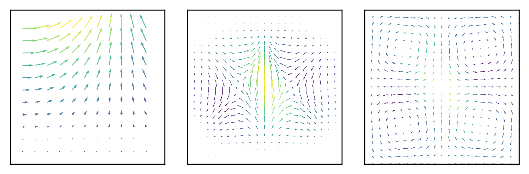
Quiver plots with color
Next, let's add some color to the quiver plots. The ax.quiver() method has an optional fifth positional argument that specifies the quiver arrow color. The quiver arrow color argument needs to have the same dimensions as the position and direction arrays.
x = np.arange(0,2.2,0.2)
y = np.arange(0,2.2,0.2)

X, Y = np.meshgrid(x, y)
u = np.cos(X)*Y
v = np.sin(y)*Y

n = -2
color_array = np.sqrt(((v-n)/2)**2 + ((u-n)/2)**2)

fig, ax = plt.subplots(figsize=(7,7))
ax.quiver(X,Y,u,v, color_array, alpha=0.8)

ax.xaxis.set_ticks([])
ax.yaxis.set_ticks([])
ax.axis([-0.2, 2.3, -0.2, 2.3])
ax.set_aspect('equal')

plt.show()

Let's add some color to the gradient quiver plot:
x = np.arange(-2,2.2,0.2)
y = np.arange(-2,2.2,0.2)


X, Y = np.meshgrid(x, y)
z = X*np.exp(-X**2 -Y**2)
dx, dy = np.gradient(z)

n = -2
color_array = np.sqrt(((dx-n)/2)**2 + ((dy-n)/2)**2)

fig, ax = plt.subplots(figsize=(7,7))
ax.quiver(X,Y,dx,dy,color_array)

ax.xaxis.set_ticks([])
ax.yaxis.set_ticks([])
ax.set_aspect('equal')

plt.show()

Finally, we'll add some color to the vortex plot:
x = np.arange(0,2*np.pi+2*np.pi/20,2*np.pi/20)
y = np.arange(0,2*np.pi+2*np.pi/20,2*np.pi/20)

X,Y = np.meshgrid(x,y)

u = np.sin(X)*np.cos(Y)
v = -np.cos(X)*np.sin(Y)

n = -1
color_array = np.sqrt(((dx-n)/2)**2 + ((dy-n)/2)**2)

fig, ax = plt.subplots(figsize=(7,7))

ax.quiver(X,Y,u,v,color_array, scale=17)

ax.xaxis.set_ticks([])
ax.yaxis.set_ticks([])
ax.axis([0,2*np.pi,0,2*np.pi])
ax.set_aspect('equal')

plt.show()

Summary
In this post, we built a couple different quiver plots with matplotlib and Python. Quiver plots are part of matplotlib's pylot library. The ax.quiver() method accepts four positional arguments: x-positions, y-positions, x-directions, y-directions. Numpy's meshgrid() function is useful for creating these position arrays. Finally, we added some color to our quiver plots by including a fifth positional argument to the ax.quiver() method.