In this post, we will complete a problem that might come up in an introductory Materials Science and Engineering class. We'll calculate the number of vacancy defects in a material using Python.

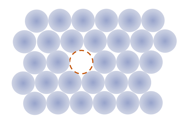
The following is a calculation of the number of vacancy defects in a material. All crystalline and poly-crystalline materials at temperatures above absolute zero contain vacancy defects. We can calculate the number of vacancies present in a material using the vacancy concentration equation below:

$$ \frac{n_v}{n} = e^{\frac{-Q_v}{RT}} $$

Where $n_v$ is the number of vacancies, $n$ is the number of potential vacancy sites, $e$ is Euler's Number (the mathematical constant $e$), $Q_v$ is the activation energy of vacancy formation, $R$ is the universal gas constant and $T$ is the temperature (in Kelvin).

The problem we are going to solve using the vacancy concentration equation is shown below.

Given:¶

A sample of 1 m³ of Cu (copper) is at 1000 °C

Density $\rho$ = 8.4 g/cm³

Activation energy of vacancy formation $Q_v$ = 86.7 kJ/mol

Molar mass of Cu $A$ = 63.5 g/mol

Avagodro's Number $N_a$ = 6.02 × 10²³ atoms/mol

Universal Gas Constant $R$ = 8.31 J/mol K

Find:¶

Find the equalibrium number of vacancies in 1 m³ of Cu at 1000 °C.

Solution:¶

Let's begin our solution by looking at the vacancy concentration equation.

$$ \frac{n_v}{n} = e^{\frac{-Q_v}{RT}} $$

We can use the vacancy concentration equation to solve for the number of vacancies $n_v$.

$$ n_v = ne^{\frac{-Q_v}{RT}} $$

We have values for: $Q_v$, $R$ and $T$. But we still need to calculate $n$, the number of potential defect sites. After we calculate $n$, we can use the equation above to calculate $n_v$. We'll start our first bit of Python code by including imports.

Imports¶

We are going to have to use Python's exp function, which raises $e$ to a power, to solve this problem. The exp function is part of Python's math module and is included in the Python Standard Library.

In Python programs, the common convention is to list imports at the top of the script. The line below imports the exp function from the math module.

In [1]:

from math import exp

Find the number of copper atoms in 1 m³ of copper¶

In order to find the number of copper atoms in 1 m³ of copper, we need to make an assumption. Let's assume that $n$, the number of potential defect sites, is approximately equal to the number of copper atoms in the sample total.

This assumption could turn out to be problematic. Copper at room temperature does contain defects, so the number of atoms isn't exactly the same as the number of potential defect sites. However, our given parameters only have 2 or 3significant figures. If the number of copper atoms and the number of potential defect sites is equivalent within 2 or 3 significant figures, our assumption will hold for this problem.

In order to find $n$ the number of copper atoms in 1 m³ of copper we need to convert 1 m³ of copper into the number of cm³ of copper using the conversion factor 1 m = 100 cm.

Next, we can calculate the number of grams of copper using the density of copper, $\rho$, given in the problem.

After that, we can use the molar mass of copper, $A$, given in the problem, to calculate the number of moles of copper.

Finally, we can calculate the number of atoms of copper $n$, using Avagadro's Number, $Na$.

The calculation is completed below in Python.

In [2]:

# find the number of atoms of copper using the volume of copper, molar mass of copper the density and avagadros number

v_Cu_m3 = 1    # volume of Cu in m^3
v_Cu_cm3 = v_Cu_m3*(100**3/1**3)  # volume of Cu in cm^3
p = 8.4 # density of Cu in g/cm3
m_Cu_g = v_Cu_cm3 * (p)  # mass of Cu in g
A = 63.5 # g/mol   molar mass of Cu from the periodic table
mol_Cu = m_Cu_g/A   # mol of Cu
Na = 6.02 * 10**23 # Avagadros Number, atoms/mol    
atoms_Cu = mol_Cu * Na  # number of atoms Cu
n = atoms_Cu # number of potential defect sites is the number of Cu atoms
print(n)

7.963464566929133e+28

This means the number of potential defect sites in 1 m³ of copper is 7.963464566929133e+28. That's a lot of potential sites for defects.

Find the number of vacancy defects in 1 m³ of copper¶

Now we have all of the values we need to calculate the number of vacancy defects in 1 m³ of copper using the equation below:

$$ n_v = ne^{\frac{-Q_v}{RT}} $$

We just need to be careful with units. In the Given portion of this problem, $Q_v$ the activation energy of vacancy formation, has units of kJ/mol. The Universal Gas constant $R$, given in the problem has units of J/mol K. And the temperature $T$ given in the problem is in units of °C. In order for the expression below (which is the exponent of the equation above) to end up unitless:

$$ \frac{-Q_v}{RT} $$

We need to convert $Q_v$ into units of J/mol K and convert $T$ into units of Kelvin. Then we can plug the values into the vacancy concentration equation and make our final calculation.

In [3]:

# find the number of vacancies, n_v using number of atoms n, Qv, R, and T
# n_v = ne^(-Qv/RT)

Qv_kJpermol =  86.7  # activation energy of vacancy formation in kJ/mol   
Qv = Qv_kJpermol*1000  # activation energy of vacancy formation in J/mol
R = 8.31  # Universal Gas Constant in J/mol K
T_C = 1000  # Temperature in *C
T = T_C+273  # Temperature in K

n_v = n*exp(-Qv/(R*T))  # number of vacancies, unitless
print(n_v)

2.1964692178195925e+25

Great! The number of vacancies in 1 m³ of copper is 2.1964692178195925e+25. That's a pretty big number, but it is three orders of magnitude less than the number of potential defect sites. We are almost done. All we need to do now is round our answer to the proper number of significant figures and print it out.

Round to the proper number of significant figures and print out the final answer¶

The last thing we need to do is round the final answer to the proper number of significant figures (sig figs). If we look back at the given values in our problem, we can determine the number of significant figures in each known parameter:

Temperature $T$ = 1000 °C - 1,2,3 or 4 sig figs

Density $\rho$ = 8.4 g/cm³ - 2 sig figs

Activation energy of vacancy formation $Q_v$ = 86.7 kJ/mol - 3 sig figs

Molar mass of Cu $A$ = 63.5 g/mol - 3 sig figs

Avagodro's Number $N_a$ = 6.02 × 10²³ atoms/mol - 3 sig figs

Universal Gas Constant $R$ = 8.31 J/mol K - 3 sig figs

The minimum number of significant figures is in the Density $\rho$ = 8.4 g/cm³ - 2 sig figs. Therefore, we will round our final answer to 2 significant figures.

We can print out our final answer using a Python f-string. Note how the character f' ' is added before the quotation marks. A little trick in the code below is in the expression:

{n_v:.1e}

Since the expression is inside a set of curly braces of an f-string, the value of the variable n_v will be printed out. The :.1e after the variable is a bit of string formating. It specifies one number after the decimal point (.1) and scientific notation e. The result is our final answer printed to 2 significant figures.

In [4]:

print(f'The number of vacancies in 1 m^3 of Cu at 1000*C is: {n_v:.1e}')

The number of vacancies in 1 m^3 of Cu at 1000*C is: 2.2e+25

Conclusion¶

In this problem, we calculated the equilibrium number of vacancies in 1 m³ of copper at 1000 °C.

We completed the problem by first calculating the number of atoms in 1 m³ of copper using density and molar mass. Then we assumed the number of atoms in 1 m³ is approximately equal to the number of potential atomic vacancy sites in 1 m³. Finally, we used the number of potential defect sites to calculate the number of vacancies in 1 m³ of copper using the vacancy concentration equation.