Crank and rocker motion is one of the classic types of motion that belongs to a category of 4-bar motion. Crank and rocker motion is the type of motion that a pumpjack goes through when pumping a fluid. In this post, you'll learn how to create an animation of crank and rocker motion using Python and Matplotlib.
Set up a Python virtual environment
To start this process, we will set up a Python virtual environment.
Real Python has a good introduction to virtual environments and why to use them.
I use the Anaconda distribution of Python. The Anaconda distribution of Python comes with the very useful Anaconda Prompt. Virtual environments can be created using the Anaconda Prompt. Open the Anaconda Prompt from the Windows Start menu and enter the following commands to create a new virtual environment.
> conda create -n piston_motion python=3.8
Now that we have a new clean virtual environment with Python 3.8 installed, we need to install the necessary packages. Note that our virtual environment (piston_motion) is active and shown in parenthesis before the prompt.
> conda activate piston_motion
(piston_motion) > conda install numpy
(piston_motion) > conda install matplotlib
(piston_motion) > conda list

...

matplotlib==2.0.2
numpy==3.4.2

...
Open a text editor or code editor and create a new Python file called piston_motion.py. A good code editor to use is Visual Studio Code. Visual Studio Code is free and open source. If you installed the Anaconda distribution of Python, you had the option of installing Visual Studio Code.
Import NumPy and Matplotlib
We will start our crank_and_rocker_motion.py script by importing the necessary packages.
# crank_and_rocker_motion.py

# import necessary packages
import numpy as np
from numpy import pi, sin, cos, sqrt, absolute, arccos, arctan, sign
import matplotlib.pyplot as plt
import matplotlib.animation as animation
Define the input parameters
To model crank and rocker motion, we need three moving parts. One is the rotating crankshaft. The crankshaft rotates around a central axis with a constant radius. We'll model crankshaft rotation with a line of constant length, one end fixed at the origin and the other rotating in a circle like a hand on a clock. To model this line, we just need two points, the origin at x=0 and y=0 and the end of the line at the point x1 and y1.
We also need to define a crank radius and define the connecting rod length. We'll define the crank radius and connecting rod length constants at the top of our code. Let's also define a fixed number of rotations. Without a fixed number of rotations, our animation will run around and around indefinitely.
The rotation increment defines how fine the 'ticks' are when our crankshaft arm rotates. A 'tick' increment of 0.1 results in a smooth animation.
# input parameters
r = 0.395  # crank radius
l = 4.27  # connecting rod length
rr = 1.15 # rocker radius
d = 4.03  # center-to-center distance
rot_num = 6  # number of crank rotations
increment = 0.1  # angle incremement
over = 1  # if over = 1 --> mechanism is on top, If over = -1, mechanism on bottom
s = over / absolute(over)
Create an array of crankshaft angles
Next, we'll create an array of crankshaft rotation angles. As the crankshaft rotates in our animation, each one of these angles will be 'ticked though'.
# create the angle array, where the last angle is the number of rotations*2*pi
angle_minus_last = np.arange(0, rot_num * 2 * pi, increment)
R_Angles = np.append(angle_minus_last, rot_num * 2 * pi)
Define the fixed points of the animation
Now we need to define a couple of fixed points. The first fixed point is the center of the crankshaft, we'll define this point at the origin x=0,y=0. The second fixed point is the center of the rocker arm. The center of the rocker arm will have the coordinates x4 and y4. We'll define the center of the rocker arm at x4 = d (where d is the center-to-center distance between the crank and the rocker) and y4 = 0.
# coordinates of the crank center point : Point 1
x1 = 0
y1 = 0

# Coordinates of the rocker center point: Point 4
x4 = d
y4 = 0
Create arrays to save the crankshaft and rocker shaft endpoints
Now that the fixed points are defined, we need to create a set of empty arrays which will contain the moving points in our animation. These moving points are:
- crankshaft x-position
- crankshaft y-position
- rocker arm angles
- rocker arm x-position
- rocker arm y-position
X2 = np.zeros(len(R_Angles))  # array of crank x-positions: Point 2
Y2 = np.zeros(len(R_Angles))  # array of crank y-positions: Point 2
RR_Angle = np.zeros(len(R_Angles))  # array of rocker arm angles
X3 = np.zeros(len(R_Angles))  # array of rocker x-positions: Point 3
Y3 = np.zeros(len(R_Angles))  # array of rocker y-positions: Point 3
Calculate the crankshaft and rocker shaft endpoints
Now for the calculations. We have our constants and empty arrays set up. We will loop over each crankshaft angle according to our 'tick' increment. For each crankshaft angle, we calculate the corresponding crankshaft endpoint and the corresponding rocker arm endpoint. These two endpoints are saved in the arrays X2,Y2 and X3,Y3.
# find the crank and connecting rod positions for each angle
for index, R_Angle in enumerate(R_Angles, start=0):
    theta1 = R_Angle
    x2 = r * cos(theta1)  # x-cooridnate of the crank: Point 2
    y2 = r * sin(theta1)  # y-cooridnate of the crank: Point 2
    e = sqrt((x2 - d) ** 2 + (y2 ** 2))
    phi2 = arccos((e ** 2 + rr ** 2 - l ** 2) / (2 * e * rr))
    phi1 = arctan(y2 / (x2 - d)) + (1 - sign(x2 - d)) * pi / 2
    theta3 = phi1 - s * phi2
    RR_Angle[index] = theta3
    x3 = rr * cos(theta3) + d
    # x cooridnate of the rocker moving point: Point 3
    y3 = rr * sin(theta3)
    # y cooridnate of the rocker moving point: Point 3

    theta2 = arctan((y3 - y2) / (x3 - x2)) + (1 - sign(x3 - x2)) * pi / 2

    X2[index] = x2  # grab the crankshaft x-position
    Y2[index] = y2  # grab the crankshaft y-position
    X3[index] = x3  # grab the connecting rod x-position
    Y3[index] = y3  # grab the connecting rod y-position
Now that our constants and calculations are complete, we can work on setting up the animation.
Set up the Matplotlib figure
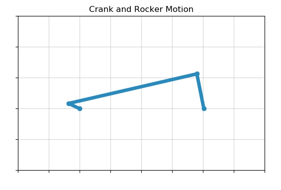
Next, we'll set up our Matplotlib figure. Note that we set aspect=equal. This parameter sets the aspect ratio of our plot as 1-to-1. Without the aspect ratio defined as 1-to-1, the crankshaft will look like an oval and the animation looks quite strange.
# set up the figure and subplot
fig = plt.figure()
ax = fig.add_subplot(
    111, aspect="equal", autoscale_on=False, xlim=(-2, 6), ylim=(-2, 3)
)

# add grid lines, title and take out the axis tick labels
ax.grid(alpha=0.5)
ax.set_title("Crank and Rocker Motion")
ax.set_xticklabels([])
ax.set_yticklabels([])
(line, ) = ax.plot(
    [], [], "o-", lw=5, color="#2b8cbe"
)  # color from: http://colorbrewer2.org/
Create an initialization function and animation function
Next, we'll create two functions. The first function init() is an initialization function and will be called at the start of our animation. The second function animate() is the animation function. This is the function that produces the animation.
# initialization function
def init():
    line.set_data([], [])
    return (line,)


# animation function
def animate(i):
    x_points = [x1, X2[i], X3[i], x4]
    y_points = [y1, Y2[i], Y3[i], y4]

    line.set_data(x_points, y_points)
    return (line,)
Call the animation and show the plot
The last part of the code is to call the animation function and show the plot. These two lines of code are the final two lines needed to make our crank and rocker animation work.
# call the animation
ani = animation.FuncAnimation(
    fig, animate, init_func=init, frames=len(X2), interval=40, blit=True, repeat=False
)
## to save animation, uncomment the line below. Ensure ffmpeg is installed:
## ani.save('crank_and_rocker_motion_animation.mp4', fps=30, extra_args=['-vcodec', 'libx264'])

# show the animation
plt.show()
Save the final changes to crank_and_rocker_motion.py. We can run our Python script from the Anaconda Prompt.
Run the animation
Run the animation by calling the crank_and_rocker_motion.py script with the Anaconda Prompt. Make sure you activate in the (piston_motion) virtual environment it is not already active.
(piston_motion) > dir
crank_and_rocker_motion.py
(piston_motion) > python crank_and_rocker_motion.py
When the animation runs you will see an example of crank and rocker motion like the video below:
Summary
In this post, we reviewed how to produce an animation of crank and rocker motion using Python and Matplotlib. First, we created a virtual environment and installed NumPy and Matplotlib into the virtual environment. Then we constructed a crank_and_rocker_motion.py script section by section. Once the crank_and_rocker_motion.py script was complete, we ran the script from the Anaconda Prompt.